pacman::p_load(tidyverse, sf, httr,
tmap)In-class Exercise 4: Preparing Spatial Interaction Modelling Variables
Overview
A healthy baby need healthy food. Likewise, a well calibrated Spatial Interaction Model need conceptually logical and well prepared propulsiveness and attractiveness variables. In this in-class exercise, you will gain hands-on experience on preparing propulsiveness and attractiveness variables require for calibrating spatial interaction models. By the end of this in-class exercise, you will be able to:
- perform geocoding by using SLA OneMap API,
- convert an aspatial data into a simple feature tibble data.frame,
- perform point-in-polygon count analysis, and
- append the propulsiveness and attractiveness variables onto a flow data.
Getting Started
To get start, the following R packages will be loaded into R environment. They are:
- tidyverse, provide a family of modern R packages for data import, wrangling
Counting number of schools in each URA Planning Subzone
Downloading General information of schools data from data.gov.sg
To get started, you are required to download General information of schools data set of School Directory and Information from data.gov.sg.
We assume that the downloaded School Directory and Information is placed in a sub-folder called data/aspatial/).
Geocoding using SLA API
Address geocoding, or simply geocoding, is the process of taking a aspatial description of a location, such as an address or postcode, and returning geographic coordinates, frequently latitude/longitude pair, to identify a location on the Earth’s surface.
Singapore Land Authority (SLA) supports an online geocoding service called OneMap API. The Search API looks up the address data or 6-digit postal code for an entered value. It then returns both latitude, longitude and x,y coordinates of the searched location.
The code chunks below will perform geocoding using SLA OneMap API. The input data will be in csv file format. It will be read into R Studio environment using read_csv function of readr package. A collection of http call functions of httr package of R will then be used to pass the individual records to the geocoding server at OneMap.
Two tibble data.frames will be created if the geocoding process completed successfully. They are called found and not_found. found contains all records that are geocoded correctly and not_found contains postal that failed to be geocoded.
Lastly, the found data table will joined with the initial csv data table by using a unique identifier (i.e. POSTAL) common to both data tables. The output data table will then save as an csv file called found.
url<-"https://www.onemap.gov.sg/api/common/elastic/search"

csv<-read_csv("data/aspatial/Generalinformationofschools.csv")
postcodes<-csv$`postal_code`

found<-data.frame()
not_found<-data.frame()

for(postcode in postcodes){
  query<-list('searchVal'=postcode,'returnGeom'='Y','getAddrDetails'='Y','pageNum'='1')
  res<- GET(url,query=query)

  if((content(res)$found)!=0){
    found<-rbind(found,data.frame(content(res))[4:13])
  } else{
    not_found = data.frame(postcode)
  }
}
Next, the code chunk below will be used to combine both found and not_found data.frames into a single tibble data.frame called merged. At the same time, we will write merged and not_found tibble data.frames into two separate csv files called schools and not_found respectively.
merged = merge(csv, found, by.x = 'postal_code', by.y = 'results.POSTAL', all = TRUE)
write.csv(merged, file = "data/aspatial/schools.csv")
write.csv(not_found, file = "data/aspatial/not_found.csv")- With the help of Google Map, located the location information of the ungeocoded school by using it’s postcode.
- Update the
results.LATITUDEandresults.LONGITUDEfields of the ungeocoded record inschoolss.csvmanually.
Tidying schools data.frame
In this sub-section, you will import schools.csv into R environment and at the same time tidying the data by selecting only the necessary fields as well as rename some fields.
Using the steps you learned in Hands-on Exercise 1, perform the following tasks:
- import schools.csv in R environment as an tibble data.frame called schools,
- rename results.LATITUDE and results.LONGITUDE to latitude and longitude respectively,
- retain only postal_code, school_name, latitude and longitude in schools tibble data.frame.
Show the code chunk
schools <- read_csv("data/aspatial/schools.csv") %>%
  rename(latitude = "results.LATITUDE",
         longitude = "results.LONGITUDE")%>%
  select(postal_code, school_name, latitude, longitude)
Converting an aspatial data into sf tibble data.frame
Next, you will convert schools tibble data.frame data into a simple feature tibble data.frame called schools_sf by using values in latitude and longitude fields.
Refer to st_as_sf() of sf package.
Show the code chunk
schools_sf <- st_as_sf(schools,
                       coords = c("longitude", "latitude"),
                       crs=4326) %>%
  st_transform(crs = 3414)
Let’s save schools_sf into an rds file by usign the code chunk below.
write_rds(schools_sf, "data/rds/schools.rds")Plotting a point simple feature layer
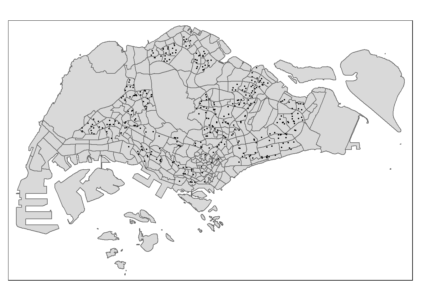
To ensure that schools sf tibble data.frame has been projected and converted correctly, you can plot the schools point data for visual inspection.
First, let us import MPSZ-2019 shapefile into R environment and save it as an sf tibble data.frame called mpsz.
Using the step your learned in previous hands-on exercise, import MPSZ-2019 shapefile into R as sf tibble data.frame and name it mpsz.
Show the code chunk
mpsz <- st_read(dsn = "data/geospatial/",
                layer = "MPSZ-2019") %>%
  st_transform(crs = 3414)
Reading layer `MPSZ-2019' from data source
`D:\tskam\ISSS624\In-class_Ex\In-class_Ex4\data\geospatial'
using driver `ESRI Shapefile'
Simple feature collection with 332 features and 6 fields
Geometry type: MULTIPOLYGON
Dimension: XY
Bounding box: xmin: 103.6057 ymin: 1.158699 xmax: 104.0885 ymax: 1.470775
Geodetic CRS: WGS 84Do it yourself!
Using the steps you learned in previous exercises, create a point symbol map showing the location of schools with OSM as the background map.
Show the code chunk
tmap_options(check.and.fix = TRUE)
tm_shape(mpsz) +
  tm_polygons() +
tm_shape(schools_sf) +
  tm_dots()
Performing point-in-polygon count process
Next, we will count the number of schools located inside the planning subzones.
Using the steps you learned from previous hands-on exercises, count the number of schools within each planning subzone by using lengths() of Base and st_intersects() of sf package.
Show the code chunk
mpsz$`SCHOOL_COUNT`<- lengths(
  st_intersects(
    mpsz, schools_sf))
It is always a good practice to examine the summary statistics of the derived variable.
Using the steps you learned in previous exercises, compute and display the summary statistics of sch_count field.
summary(mpsz$SCHOOL_COUNT) Min. 1st Qu. Median Mean 3rd Qu. Max.
0.000 0.000 0.000 1.054 2.000 12.000 The summary statistics above reveals that there are excessive 0 values in SCHOOL_COUNT field. If log() is going to use to transform this field, additional step is required to ensure that all 0 will be replaced with a value between 0 and 1 but not 0 neither 1.
Data Integration and Final Touch-up
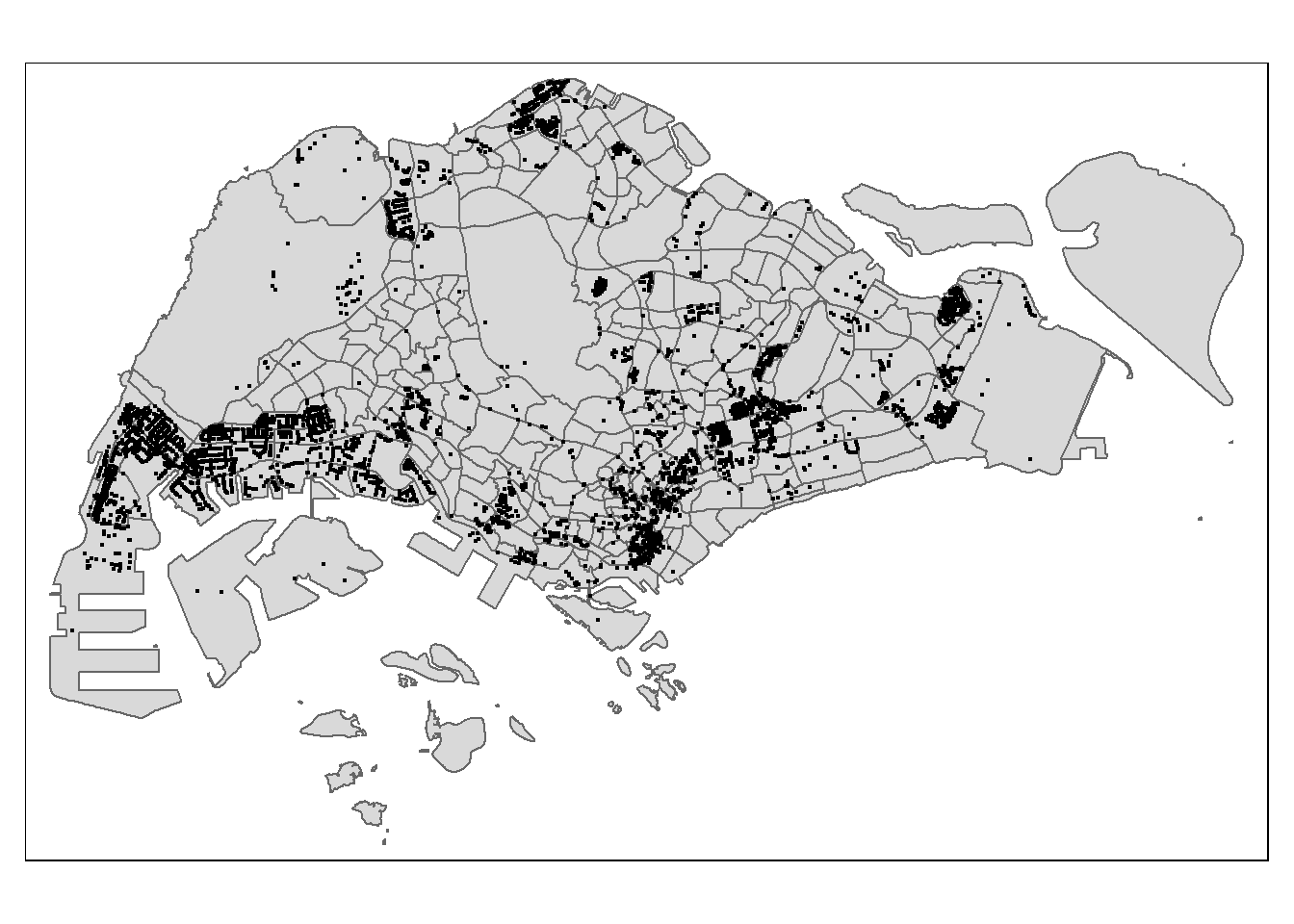
Using the steps you learned in earlier sub-sections, count the number of Business points in each planning subzone.
business_sf <- st_read(dsn = "data/geospatial",
                      layer = "Business")
Reading layer `Business' from data source
`D:\tskam\ISSS624\In-class_Ex\In-class_Ex4\data\geospatial'
using driver `ESRI Shapefile'
Simple feature collection with 6550 features and 3 fields
Geometry type: POINT
Dimension: XY
Bounding box: xmin: 3669.148 ymin: 25408.41 xmax: 47034.83 ymax: 50148.54
Projected CRS: SVY21 / Singapore TMShow the code chunk
tmap_options(check.and.fix = TRUE)
tm_shape(mpsz) +
  tm_polygons() +
tm_shape(business_sf) +
  tm_dots()
Show the code chunk
mpsz$`BUSINESS_COUNT`<- lengths(
  st_intersects(
mpsz, business_sf))summary(mpsz$BUSINESS_COUNT) Min. 1st Qu. Median Mean 3rd Qu. Max.
0.00 0.00 2.00 19.73 13.00 307.00 Now, it is time for us to bring in the flow_data.rds saved after Hands-on Exercise 3.
Show the code chunk
flow_data <- read_rds("data/rds/flow_data.rds")
flow_data
Simple feature collection with 14734 features and 10 fields
Geometry type: LINESTRING
Dimension: XY
Bounding box: xmin: 5105.594 ymin: 25813.33 xmax: 49483.22 ymax: 49552.79
Projected CRS: SVY21 / Singapore TM
First 10 features:
ORIGIN_SZ DESTIN_SZ MORNING_PEAK dist ORIGIN_AGE7_12 ORIGIN_AGE13_24
1 AMSZ01 AMSZ01 1998 50.0000 310 710
2 AMSZ01 AMSZ02 8289 810.4491 310 710
3 AMSZ01 AMSZ03 8971 1360.9294 310 710
4 AMSZ01 AMSZ04 2252 840.4432 310 710
5 AMSZ01 AMSZ05 6136 1076.7916 310 710
6 AMSZ01 AMSZ06 2148 805.2979 310 710
7 AMSZ01 AMSZ07 1620 1798.7526 310 710
8 AMSZ01 AMSZ08 1925 2576.0199 310 710
9 AMSZ01 AMSZ09 1773 1204.2846 310 710
10 AMSZ01 AMSZ10 63 1417.8035 310 710
ORIGIN_AGE25_64 DESTIN_AGE7_12 DESTIN_AGE13_24 DESTIN_AGE25_64
1 2780 310.00 710.00 2780.00
2 2780 1140.00 2770.00 15700.00
3 2780 1010.00 2650.00 14240.00
4 2780 980.00 2000.00 11320.00
5 2780 810.00 1920.00 9650.00
6 2780 1050.00 2390.00 12460.00
7 2780 420.00 1120.00 3620.00
8 2780 390.00 1150.00 4350.00
9 2780 1190.00 3260.00 13350.00
10 2780 0.99 0.99 0.99
geometry
1 LINESTRING (29501.77 39419....
2 LINESTRING (29501.77 39419....
3 LINESTRING (29501.77 39419....
4 LINESTRING (29501.77 39419....
5 LINESTRING (29501.77 39419....
6 LINESTRING (29501.77 39419....
7 LINESTRING (29501.77 39419....
8 LINESTRING (29501.77 39419....
9 LINESTRING (29501.77 39419....
10 LINESTRING (29501.77 39419....Notice that this is an sf tibble data.frame and the features are polylines linking the centroid of origins and destination planning subzone.
Using the steps your learned in Hands-on Exercise 3, append SCHOOL_COUNT and BUSINESS_COUNT into flow_data sf tibble data.frame.
Show the code chunk
mpsz_tidy <- mpsz %>%
  st_drop_geometry() %>%
  select(SUBZONE_C, SCHOOL_COUNT, BUSINESS_COUNT)
Now, we will append SCHOOL_COUNT and BUSINESS_COUNT fields from mpsz_tidy data.frame into flow_data sf tibble data.frame by using the code chunk below.
flow_data <- flow_data %>%
  left_join(mpsz_tidy,
            by = c("DESTIN_SZ" = "SUBZONE_C")) %>%
  rename(TRIPS = MORNING_PEAK,
DIST = dist)Note that the unique join field used is DESTIN_SZ of flow_data and SUBZONE_C of mpsz_tidy. Do you know why?
Checking for variables with zero values
Since Poisson Regression is based of log and log 0 is undefined, it is important for us to ensure that no 0 values in the explanatory variables.
In the code chunk below, summary() of Base R is used to compute the summary statistics of all variables in wd_od data frame.
summary(flow_data) ORIGIN_SZ DESTIN_SZ TRIPS DIST
Length:14734 Length:14734 Min. : 1 Min. : 50
Class :character Class :character 1st Qu.: 14 1st Qu.: 3346
Mode :character Mode :character Median : 76 Median : 6067
Mean : 1021 Mean : 6880
3rd Qu.: 426 3rd Qu.: 9729
Max. :232187 Max. :26136
ORIGIN_AGE7_12 ORIGIN_AGE13_24 ORIGIN_AGE25_64 DESTIN_AGE7_12
Min. : 0.99 Min. : 0.99 Min. : 0.99 Min. : 0.99
1st Qu.: 240.00 1st Qu.: 440.00 1st Qu.: 2200.00 1st Qu.: 240.00
Median : 700.00 Median : 1350.00 Median : 6810.00 Median : 720.00
Mean :1031.86 Mean : 2268.84 Mean :10487.62 Mean :1033.40
3rd Qu.:1480.00 3rd Qu.: 3260.00 3rd Qu.:15770.00 3rd Qu.:1500.00
Max. :6340.00 Max. :16380.00 Max. :74610.00 Max. :6340.00
DESTIN_AGE13_24 DESTIN_AGE25_64 SCHOOL_COUNT BUSINESS_COUNT
Min. : 0.99 Min. : 0.99 Min. : 0.000 Min. : 0.00
1st Qu.: 460.00 1st Qu.: 2200.00 1st Qu.: 0.000 1st Qu.: 0.00
Median : 1420.00 Median : 7030.00 Median : 1.000 Median : 3.00
Mean : 2290.35 Mean :10574.46 Mean : 1.583 Mean : 16.17
3rd Qu.: 3260.00 3rd Qu.:15830.00 3rd Qu.: 2.000 3rd Qu.: 12.00
Max. :16380.00 Max. :74610.00 Max. :12.000 Max. :307.00
geometry
LINESTRING :14734
epsg:3414 : 0
+proj=tmer...: 0
The print report above reveals that variables ORIGIN_AGE7_12, ORIGIN_AGE13_24, ORIGIN_AGE25_64, DESTIN_AGE7_12, DESTIN_AGE13_24, DESTIN_AGE25_64 consist of 0 values.
In view of this, code chunk below will be used to replace zero values to 0.99.
flow_data$SCHOOL_COUNT <- ifelse(
  flow_data$SCHOOL_COUNT == 0,
  0.99, flow_data$SCHOOL_COUNT)
flow_data$BUSINESS_COUNT <- ifelse(
  flow_data$BUSINESS_COUNT == 0,
  0.99, flow_data$BUSINESS_COUNT)
You can run the summary() again.
summary(flow_data) ORIGIN_SZ DESTIN_SZ TRIPS DIST
Length:14734 Length:14734 Min. : 1 Min. : 50
Class :character Class :character 1st Qu.: 14 1st Qu.: 3346
Mode :character Mode :character Median : 76 Median : 6067
Mean : 1021 Mean : 6880
3rd Qu.: 426 3rd Qu.: 9729
Max. :232187 Max. :26136
ORIGIN_AGE7_12 ORIGIN_AGE13_24 ORIGIN_AGE25_64 DESTIN_AGE7_12
Min. : 0.99 Min. : 0.99 Min. : 0.99 Min. : 0.99
1st Qu.: 240.00 1st Qu.: 440.00 1st Qu.: 2200.00 1st Qu.: 240.00
Median : 700.00 Median : 1350.00 Median : 6810.00 Median : 720.00
Mean :1031.86 Mean : 2268.84 Mean :10487.62 Mean :1033.40
3rd Qu.:1480.00 3rd Qu.: 3260.00 3rd Qu.:15770.00 3rd Qu.:1500.00
Max. :6340.00 Max. :16380.00 Max. :74610.00 Max. :6340.00
DESTIN_AGE13_24 DESTIN_AGE25_64 SCHOOL_COUNT BUSINESS_COUNT
Min. : 0.99 Min. : 0.99 Min. : 0.990 Min. : 0.99
1st Qu.: 460.00 1st Qu.: 2200.00 1st Qu.: 0.990 1st Qu.: 0.99
Median : 1420.00 Median : 7030.00 Median : 1.000 Median : 3.00
Mean : 2290.35 Mean :10574.46 Mean : 1.987 Mean : 16.47
3rd Qu.: 3260.00 3rd Qu.:15830.00 3rd Qu.: 2.000 3rd Qu.: 12.00
Max. :16380.00 Max. :74610.00 Max. :12.000 Max. :307.00
geometry
LINESTRING :14734
epsg:3414 : 0
+proj=tmer...: 0
Notice that all the 0 values have been replaced by 0.99.
Before we move on to calibrate the Spatial Interaction Models, let us save flow_data sf tibble data.frame into an rds file. Call the file flow_data_tidy.
write_rds(flow_data,
          "data/rds/flow_data_tidy.rds")